Matrix in Ebitengine
This article explains what are matrices and how they are used in Ebitengine. We don't explain a strict mathematical theory. Instead, we explain essential knowledge for Ebitengine.
TL;DR
Ebitengine uses a mathematical matrix to specify how an image is transformed geometrically like scaling or rotating. A combination of multiple geometric transforms can be represented by one matrix.
Coordinate System
Ebitengine treats 2D graphics, and defines its coordinate system. X axis is rightward, and Y axis is downward. The origin point is upper left.
The coordinate system exists for each ebiten.Image object. The upper left point of the destination image is the origin point of the coordinate system.

Matrix
ebiten.Image is a set of pixels on a 2D rectangle. In Ebitengine, you can apply a conversion rule for each pixel. By the conversion rule, you can put an image at a specified position, and you can also apply various effects like scaling or rotating. As a conversion rule, Ebitengine uses a matrix.
In 2D space, a point is represented as a 2D vector (x, y). A 2D matrix converts this and generates a new point.

Definition
A matrix is a mathematical value used in linear algebra. A matrix is an array of numbers. A 2D matrix is like this.
\begin{aligned} \begin{bmatrix} 0.5000 & -0.8660 \\ 0.8660 & 0.5000 \\ \end{bmatrix} \end{aligned}
The horizontal sequences are called rows, and the vertical sequences are called columns. If the size is 2, the matrix is called 2D (two-dimensional) matrix, and if 3, 3D (three-dimensional) matrix. A 3D matrix is like this.
\begin{aligned} \begin{bmatrix} 0.2990 & 0.5870 & 0.1140 \\ -0.1687 & -0.3313 & 0.5000 \\ 0.5000 & -0.4187 & -0.0813 \\ \end{bmatrix} \end{aligned}
If the numbers of columns and rows are the same, the matrix is called a regular matrix. Ebitengine treats only regular matrices.
Multiplying a matrix and a vector
You can multiply a matrix and a vector. The matrix is on the left side and the vector is on the right side. In general mathematics, the swapped positions are also possible but Ebitengine doesn't treat the swapped positions.
A matrix is a conversion rule, and in the equation, (x, y) means a point before converting, multiplying means applying the conversion rule, and (ax+by, cx+dy) means a point after converting.
\begin{aligned} \begin{bmatrix} a & b \\ c & d \\ \end{bmatrix} \begin{bmatrix} x \\ y \\ \end{bmatrix} = \begin{bmatrix} ax + by \\ cx + dy \\ \end{bmatrix} \end{aligned}
By the way, this is the same in the three-dimensional case.
\begin{aligned} \begin{bmatrix} a & b & c \\ d & e & f \\ g & h & i \\ \end{bmatrix} \begin{bmatrix} x \\ y \\ z \\ \end{bmatrix} = \begin{bmatrix} ax + by + cz \\ dx + ey + fz \\ gx + hy + iz \\ \end{bmatrix} \end{aligned}
Identity matrix
An identity matrix is a matrix that doesn't change the multiplicand.
\begin{aligned} \begin{bmatrix} 1 & 0 \\ 0 & 1 \\ \end{bmatrix} \end{aligned}
Let's multiply this identity matrix and a vector. You can confirm that the input and the output are the same. This matrix doesn't change any points on a 2D space.
\begin{aligned} \begin{bmatrix} 1 & 0 \\ 0 & 1 \\ \end{bmatrix} \begin{bmatrix} x \\ y \\ \end{bmatrix} = \begin{bmatrix} 1 \cdot x + 0 \cdot y \\ 0 \cdot x + 1 \cdot y \\ \end{bmatrix} = \begin{bmatrix} x \\ y \\ \end{bmatrix} \end{aligned}
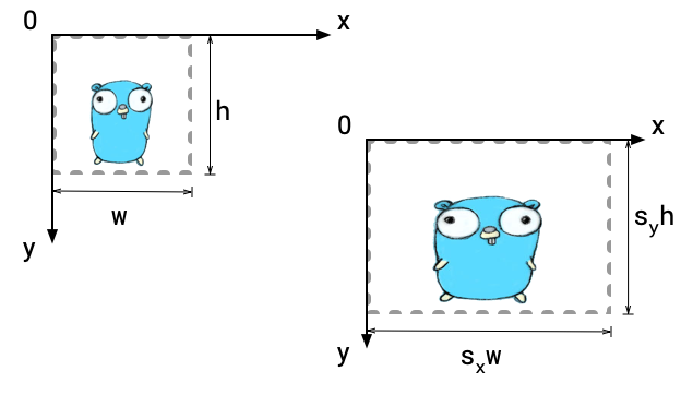
Scaling
A matrix that scales an image by s_x times in X direction and by s_y times in Y direction centering at the origin is this.
\begin{aligned} \begin{bmatrix} s_x & 0 \\ 0 & s_y \\ \end{bmatrix} \end{aligned}
Let's multiply this matrix and a vector.
\begin{aligned} \begin{bmatrix} s_x & 0 \\ 0 & s_y \\ \end{bmatrix} \begin{bmatrix} x \\ y \\ \end{bmatrix} = \begin{bmatrix} s_x \cdot x + 0 \cdot y \\ 0 \cdot x + s_y \cdot y \\ \end{bmatrix} = \begin{bmatrix} s_x x \\ s_y y \\ \end{bmatrix} \end{aligned}
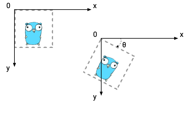
Rotating
A matrix that rotates an image by an angle \theta centering at the origin is this. This uses trigonometric functions. Please don't worry if you don't know trigonometric functions. Ebitengine has a useful function to rotate images.
\begin{aligned} \begin{bmatrix} \cos \theta & -\sin \theta \\ \sin \theta & \cos \theta \\ \end{bmatrix} \end{aligned}
Multiplying a matrix and a matrix
For example, what if you want to combine scaling and rotating? To come to the point, such combinations of conversion rules can be represented as one matrix. Let's see how two matrices are combined.
If a vector is multiplied by two matrices, the equation will be like this.
\begin{aligned} \begin{bmatrix} a_2 & b_2 \\ c_2 & d_2 \\ \end{bmatrix} \begin{bmatrix} a_1 & b_1 \\ c_1 & d_1 \\ \end{bmatrix} \begin{bmatrix} x \\ y \\ \end{bmatrix} &= \begin{bmatrix} a_2 & b_2 \\ c_2 & d_2 \\ \end{bmatrix} \begin{bmatrix} a_1 x + b_1 y \\ c_1 x + d_1 y \\ \end{bmatrix} \\ &= \begin{bmatrix} a_2(a_1 x + b_1 y) + b_2(c_1 x + d_1 y) \\ c_2(a_1 x + b_1 y) + d_2(c_1 x + d_1 y) \\ \end{bmatrix} \\ &= \begin{bmatrix} a_2 a_1 x + a_2 b_1 y + b_2 c_1 x + b_2 d_1 y \\ c_2 a_1 x + a_2 b_1 y + d_2 c_1 x + d_2 d_1 y \\ \end{bmatrix} \\ &= \begin{bmatrix} a_2 a_1 x + b_2 c_1 x + a_2 b_1 y + b_2 d_1 y \\ c_2 a_1 x + d_2 c_1 x + a_2 b_1 y + d_2 d_1 y \\ \end{bmatrix} \\ &= \begin{bmatrix} (a_2 a_1 + b_2 c_1) x + (a_2 b_1 + b_2 d_1) y \\ (c_2 a_1 + d_2 c_1) x + (c_2 b_1 + d_2 d_1) y \\ \end{bmatrix} \\ &= \begin{bmatrix} a_2 a_1 + b_2 c_1 & a_2 b_1 + b_2 d_1 \\ c_2 a_1 + d_2 c_1 & c_2 b_1 + d_2 d_1 \\ \end{bmatrix} \begin{bmatrix} x \\ y \\ \end{bmatrix} \end{aligned}
What an intimidating equation! However, this is a very beautiful result. This equation means that we can define multiplying two matrices like this.
\begin{aligned} \begin{bmatrix} a_2 & b_2 \\ c_2 & d_2 \\ \end{bmatrix} \begin{bmatrix} a_1 & b_1 \\ c_1 & d_1 \\ \end{bmatrix} = \begin{bmatrix} a_2 a_1 + b_2 c_1 & a_2 b_1 + b_2 d_1 \\ c_2 a_1 + d_2 c_1 & c_2 b_1 + d_2 d_1 \\ \end{bmatrix} \end{aligned}
Then, we were able to define the combination of two conversions as another matrix.
You don't have to remember this equation, but please remember the fact that multiplying two matrices results in one matrix.
By the way, in three-dimensional cases, multiplying will be like this.
\begin{aligned} & \begin{bmatrix} a_2 & b_2 & c_2 \\ d_2 & e_2 & f_2 \\ g_2 & h_2 & i_2 \\ \end{bmatrix} \begin{bmatrix} a_1 & b_1 & c_1 \\ d_1 & e_1 & f_1 \\ g_1 & h_1 & i_1 \\ \end{bmatrix} \\ =& \begin{bmatrix} a_2 a_1 + b_2 d_1 + c_2 g_1 & a_2 b_1 + b_2 e_1 + c_2 h_1 & a_2 c_1 + b_2 f_1 + c_2 i_1 \\ d_2 a_1 + e_2 d_1 + f_2 g_1 & d_2 b_1 + e_2 e_1 + f_2 h_1 & d_2 c_1 + e_2 f_1 + f_2 i_1 \\ g_2 a_1 + h_2 d_1 + i_2 g_1 & g_2 b_1 + h_2 e_1 + i_2 h_1 & g_2 c_1 + h_2 f_1 + i_2 i_1 \\ \end{bmatrix} \end{aligned}
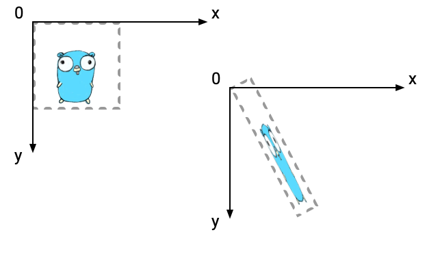
Be careful that the order of multiplying matters. If there is a matrix A and a matrix B, the results of AB and BA are different in general. For example, \big[\begin{smallmatrix}1&2\\3&4\end{smallmatrix}\big]\big[\begin{smallmatrix}5&6\\7&8\end{smallmatrix}\big] is different from \big[\begin{smallmatrix}5&6\\7&8\end{smallmatrix}\big]\big[\begin{smallmatrix}1&2\\3&4\end{smallmatrix}\big]. In the context of conversion rule, rotating and scaling an image in this order is different from scaling and rotating the image in this order in general.
\begin{aligned} \begin{bmatrix} 1 & 2 \\ 3 & 4 \\ \end{bmatrix} \begin{bmatrix} 5 & 6 \\ 7 & 8 \\ \end{bmatrix} &= \begin{bmatrix} 19 & 22 \\ 43 & 50 \\ \end{bmatrix} \\ \begin{bmatrix} 5 & 6 \\ 7 & 8 \\ \end{bmatrix} \begin{bmatrix} 1 & 2 \\ 3 & 4 \\ \end{bmatrix} &= \begin{bmatrix} 23 & 34 \\ 31 & 46 \\ \end{bmatrix} \\ \begin{bmatrix} 1 & 2 \\ 3 & 4 \\ \end{bmatrix} \begin{bmatrix} 5 & 6 \\ 7 & 8 \\ \end{bmatrix} &\ne \begin{bmatrix} 5 & 6 \\ 7 & 8 \\ \end{bmatrix} \begin{bmatrix} 1 & 2 \\ 3 & 4 \\ \end{bmatrix} \end{aligned}
Affine transformation
A 2D matrix looks enough to move points, but there is a problem. Any 2D matrices cannot move the origin point (0, 0).
\begin{aligned} \begin{bmatrix} a & b \\ c & d \\ \end{bmatrix} \begin{bmatrix} 0 \\ 0 \\ \end{bmatrix} = \begin{bmatrix} a \cdot 0 & b \cdot 0 \\ c \cdot 0 & d \cdot 0 \\ \end{bmatrix} = \begin{bmatrix} 0 \\ 0 \\ \end{bmatrix} \end{aligned}
So can't we represent translating by matrices?
Then, we introduce an affine transform matrix. For 2D vectors, an affine transform matrix is like this. The matrix is extended to be three-dimensional. The last row is always (0, 0, 1).
\begin{aligned} \begin{bmatrix} a & b & t_x \\ c & d & t_y \\ 0 & 0 & 1 \\ \end{bmatrix} \end{aligned}
The vector will also be extended to three dimensional, and the third value is always 1. A 2D vector (x, y) will be (x, y, 1).
\begin{aligned} \begin{bmatrix} x \\ y \\ 1 \\ \end{bmatrix} \end{aligned}
Let's multiply this affine transform matrix and the extended vector. You can confirm that the result includes new terms t_x and t_y.
\begin{aligned} \begin{bmatrix} a & b & t_x \\ c & d & t_y \\ 0 & 0 & 1 \\ \end{bmatrix} \begin{bmatrix} x \\ y \\ 1 \\ \end{bmatrix} = \begin{bmatrix} a \cdot x + b \cdot y + t_x \cdot 1 \\ c \cdot x + d \cdot y + t_y \cdot 1 \\ 0 \cdot x + 0 \cdot y + 1 \cdot 1 \\ \end{bmatrix} = \begin{bmatrix} ax + by + t_x \\ cx + dy + t_y \\ 1 \\ \end{bmatrix} \end{aligned}
Translating
A matrix that just translates an image is this.
\begin{aligned} \begin{bmatrix} 1 & 0 & t_x \\ 0 & 1 & t_y \\ 0 & 0 & 1 \\ \end{bmatrix} \end{aligned}
Let's apply this matrix to a vector (x, y, 1). The result is translating x and y by t_x and t_y respectively.
\begin{aligned} \begin{bmatrix} 1 & 0 & t_x \\ 0 & 1 & t_y \\ 0 & 0 & 1 \\ \end{bmatrix} \begin{bmatrix} x \\ y \\ 1 \\ \end{bmatrix} = \begin{bmatrix} 1 \cdot x + 0 \cdot y + t_x \cdot 1 \\ 0 \cdot x + 1 \cdot y + t_y \cdot 1 \\ 0 \cdot x + 0 \cdot y + 1 \cdot 1 \\ \end{bmatrix} = \begin{bmatrix} x + t_x \\ y + t_y \\ 1 \\ \end{bmatrix} \end{aligned}
![]()
Scaling and rotating matrix we already explained will be a matrix that t_x and t_y are 0.
We don't prove this here, but multiplying two affine transform matrices results in an affine transform matrix. This means that any combinations of scaling, rotating and translating are represented as one affine transform matrix. Based on this fact, Ebitengine's API for geometric transform is very simple and requires only one affine transform matrix. Ebitengine's matrices are always affine transform, and doesn't treat other matrices.
Filter
We explained that converting an image is represented by a matrix that moves each pixel of the image. You might already realize this, but as a matter of fact, enlarging an image in this way results in an image with full of holes, since the destination area is larger than the source area. To avoid such odd results, Ebitengine complements pixels by filters. The way in which the pixels are complemented is determined by a filter type, like ebiten.FilterNearest or ebiten.FilterLinear
Color matrix
In Ebitengine, matrices are also used when converting colors. We don't explain details here. Ebitengine treats an RGBA color as a point in 4D space, and convert it with a matrix. The matrix is an affine transform matrix, and the dimension is 5.
\begin{aligned} \begin{bmatrix} x_1 & x_2 & x_3 & x_4 & t_r \\ x_5 & x_6 & x_7 & x_8 & t_g \\ x_9 & x_{10} & x_{11} & x_{12} & t_b \\ x_{13} & x_{14} & x_{15} & x_{16} & t_a \\ 0 & 0 & 0 & 0 & 1 \\ \end{bmatrix} \begin{bmatrix} r \\ g \\ b \\ a \\ 1 \\ \end{bmatrix} \end{aligned}